Fading channel modeling is a fairly common step while performing any communication system analysis. This article deals with how to model a fading channel with the assumption that channel taps are sample spaced. The first section tells what are the sample spaced taps of the channel and next the discussion is about how can we model such channel in MATLAB along with an example script.
What does it mean by "sampled spaced taps"? Suppose you have the simplest communication system perspective consisting of a transmitter, channel and receiver where the transmitted waveform passes through the channel and is received by the receiver after getting reflected from different obstacles. While modeling we need to discretize the channel so that it can be simulated in MATLAB or any simulation environment i.e. take channel response at particular time instants and not all the time. So a discrete channel is defined by a set of impulses at particular instant of time instead of a continuous response. These impulses at particular instants are called channel taps and every tap corresponds to a seperate reflected wave that comes after some delay. Quite intuitively, there is no binding on the lengths of paths that these reflected waves travel so there is no binding on how delayed these reflected signals will be received. For example, the second wave can come after a span of 1 microseconds of the first wave and the third wave can come after 2.3 microseconds of the second wave. By sample spaced channel taps, we mean that the difference in delays between different waves is either some sampling interval Ts or a multiple of it.

Now, to model the first channel is quite difficult as compared to the second one because the second channel can easily be implemented using a 3-tap FIR filter as the sampling frequency is fixed.
So, this is quite apparent that if we want to model such channel using an FIR filter i.e. assuming sample spaced taps, we will have to input the waveform samples (that comes out of the transmitter) with the same sampling interval as that of the time interval between the FIR channel taps. With this assumption, we cannot simulate a channel where taps are not uniformly spaced. For this, we will have to interpolate the input wave and/or the channel response. This will be discussed in the next section of this tutorial. In this article, we consider only the case where channel taps are sample spaced i.e. the time interval (or 1/Sampling Frquency) of the signal is the same as that of channel.
All right! We are now ready to simulate the whole process. Lets take an example of modeling the following channel to clarify the whole picture.
Channel Specifications
- No. of Taps = 4
- No. of Independent Channel Responses = 2000
- Tap Weights and Delays
- First Tap = 0 dB with delay of 0 microseconds
- Second Tap = -5 dB with delay of 5 microseconds
- Third Tap = -10 dB with delay of 10 microseconds
- Fourth Tap = -15 dB with delay of 15 microseconds
- The sampling frequency of the input signal = 1/5 microseconds = 200 kHz
This channel is sample spaced because,
sampling interval of input signal = 5 microseconds = Mx(delay difference between two consecutive taps) where M = 1.
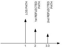
The channel is depicted in the following figure.

First we will make 4 independantly rayleigh faded channel taps. This can be easily done by using the fact that the envelope of two gaussian processes with the same variance and mean is rayleigh distributed. One can make a rayleigh faded tap quite easily using following equation and code in MATLAB.
---------------------------------------------------------------
%% MATLAB Code
no_of_taps = 4;
averaging_interval = 2000;
tap_weights_db = [0 -5 -10 -15];
tap_delays = [0 5e-6 10e-6 15e-6];
% Conversion of dBs scale into linear one
tap_weights_ln = 10.^(tap_weights_db/10);
% Calculation of normalization factor to make the average power of output
% signal to 1
norm_fact = sqrt(sum(tap_weights_ln));
% Generating a Rayleigh Random Variable with average power 1
taps = 1/sqrt(2)*(randn(averaging_interval, no_of_taps) + j*randn(averaging_interval,no_of_taps));
% Making average power of different taps to specified value
taps_weights = taps.*repmat(sqrt(tap_weights_ln), averaging_interval,1);
% Applying to normalization factor
taps_norm = 1/norm_fact*taps_weights;
---------------------------------------------------------------
Normalization Factors
In the above code, there are two normalization factors involved.
| 1. | |
| 2. | norm_fact |
The need for these normalization factors arise due to the following reason. When we talk about different taps, actually different replicas of the signal is being added with different delays. The result is that the output signal from this multipath channel has power more than what was input to the channel. For example, if we have input a signal of power 1, the output of channel shouldn't at least exceed a power of 1. That's why the tap values are scaled so as to make the total output power equal to 1 for an input signal of power 1 while adding all the replicas. Further, every tap is also a summation of two signals in quadrature each with variance (average normalized power in the AC component) equal to 1. In summary, we need normalization at two stages.
- To make average normalized power of rayleigh faded process equal to 1.
- To make average normalized power of all the rayleigh faded taps equal to 1.
In fact, both of these normalization process can be combined as for 2nd normalization we are assuming that each tap has power 1.
The very first question now arises what is the power of two normally distributed processes added in quadrature? This can be perceived as follows. The randn command creates a gaussian distributed random variable with zero mean and variance 1. Since, variance represents the average normalized power in the AC (varying) component of the signal, we can say that randn will create a gaussian distributed random variable with 0 DC value and 1 average normalized power in AC component. So, we know that the AC power of the two normally distributed R.Vs added in quadrature is 2 with an amplitude of sqrt(2). To make this signal with amplitude sqrt(2) into a signal of amplitude 1 (that will give in return a power of 1^2 = 1), we need to divide the signal with sqrt(2). That's all about the first normalization factor. It just makes the average normalized power in the AC-component of two normally distributed R.V.s added in quadrature to a value of 1.
The same analogy can be applied to the understanding of 2nd scaling factor. We needed first scaling factor because we were adding two signals each of power 1. Now, each tap represents a signal of power 1 and they are being added with different weights (and thus different average powers) to each other to produce the effect of multipath. In our case, the same signal is added 4 times (because of the 4 taps) and the average output power is equal to the sum of average powers of the four taps. As described in the channel specification, the power of different taps is as follows.
- First Tap = 0 dB or 1 with delay of 0 microseconds
- Second Tap = -5 dB or 0.316 with delay of 5 microseconds
- Third Tap = -10 dB or 0.1 with delay of 10 microseconds
- Fourth Tap = -15 dB or 0.0316 with delay of 15 microseconds
Thus, the total output power of this channel is 1+0.316+.1+0.0316 = 1.447. If we input a signal of average power 1 to this channel, the average power of the output of the channel would be 1.447. To make the average power of the output signal to 1, we need to divide the taps by sqrt(1.447) = sqrt(sum of linear values of the taps) as done in the code. In summary, both of these normalization factors were incorporated to make the average output power of the channel equal to 1 for a signal of input power 1.
Generating The Taps
Finally, all the taps are generated using these normalizations and two independent gaussian random variables. Following is the code that proves that the average normalized power of different taps is as specified in the channel.
---------------------------------------------------------------
%% MATLAB Code
disp('The path gains are as follows (in dB)');
20*log10(mean(abs(taps_norm),1))
disp('The total path gain of the channel is');
sum(mean(abs(taps_norm).^2,1))
---------------------------------------------------------------
The complete MATLAB script can be found here.
The physical meanings of different statistical parameters such as mean, variance etc. are given in chapter-1 of Digital Communications: Fundamentals and Applications (2nd Edition) (Prentice Hall Communications Engineering and Emerging Technologies Series).

